
WASSA 2023 Shared Task on Empathy Detection and Emotion Classification and Personality Detection in Interactions
TransformerRoBERTa Fine-TuningEmpathy ClassificationText ClassificationNatural Language ProcessingTrack 1: Empathy and Emotion Prediction in Conversations (CONV)
Team Members:
- Sushant Karki
- Xiaoyan Feng
- Vladimir Rife
Introduction:
The task our group set out to solve was WASSA’s 2023 Shared Task on Empathy Emotion and Personality Detection in Interactions Track 1: Empathy and Emotion Prediction in Conversations. The goal of our problem was to predict the measure of emotional polarity (negative/positive emotion), emotional intensity (strength of that emotion), and empathy towards an article topic discussed in conversations between participants of WASSA’s 2023 data collection experiment. The purpose of solving this problem is to better quantify the type, intensity, and interpersonal effects of emotion as communicated through natural language like the conversations from WASSA’s experiment. If a reliable algorithm trained on such conversations could be applied to any human text, we might be able to advance many fields of science and technology like chatbots, mood-tracking, therapy, medical diagnoses, behavioral prediction, etc.
Dataset:
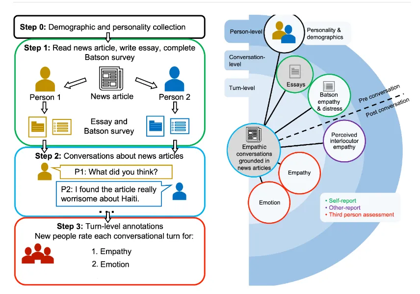
The dataset WASSA provided for their shared tasks was collected in 4 stages (visual figure given below). In Stage 0, they collected demographic and personality data on the participants and recorded it. In Stage 1, those participants were told to read one of their finite number of news articles and write their reaction to it down in the form of a 300-800 character essay and Batson survey. In Stage 2, participants who had read the same article were paired together to have a recorded conversation about it. And then, in Stage 3, annotators went through the recorded text of those conversations on a turn-by-turn basis and evaluated the emotional polarity, emotional intensity, and empathy the participant showed toward the article subject on a [0,2] scale for emotional polarity and [0,5] scale for emotional intensity and empathy. It is also important to note that the emotional polarity, emotional intensity, and empathy scores are not continuous values within their given ranges, but rather, discrete values in increments of thirds within them (so, ⅓, ⅔, 1, 4/3, and so on…).
Baseline Model(s) and Performance Metrics:
The initial baseline model we chose by which to measure the rest of our models up against was a One-vs-rest (OvR) Logistic Regression model. OvR logistic regression is a type of binary classification algorithm in which a single class is compared against all other classes in a multi-class classification problem, by training one binary logistic regression classifier for each class to distinguish it from the rest of the classes. The metrics we used to measure the performance of the baseline model, and all our other models, were their Accuracy, F1 scores, and Pearson R scores. We chose these metrics because accuracy demonstrates the proportion of correctly classified instances over the total number of instances across all classes, F1-score provides a balanced measure (via the harmonic mean between precision and recall) of the model's ability to correctly identify positive instances and avoid false negatives, and the Pearson R score demonstrates the strength and direction of the linear relationship between the predicted and actual values, providing a good indication of how well the model’s prediction fits the data’s true labels. As we can see in the figures and table assessing these metrics in our baseline model below, the results are not as good as we would like (none of the scores meaningfully reach above a value of 0.5). But, this is to be expected in a baseline. The following sections will show how we improve upon this.
Baseline model for Emotional Polarity:
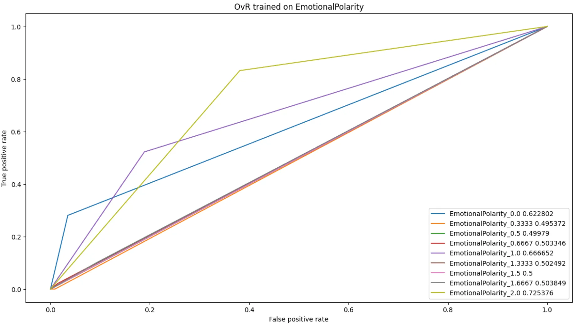
From the figure, we can clearly find that the category of score 2 has the best ROC curve; the category of score 1 is the second one; 0 is the third. Other than these three categories, they all overlap at the diagonal of this Coordinate System, which shows that this OvR cannot distinguish these categories. As far as we can see, the reason for this phenomenon is caused by the unbalance of the data, and implies that the smaller the difference of labels are, the harder the model could classify. The trials of label smoothing and generating similar data in the Emotional Polarity model are based on these findings.
Baseline model for Emotional Intensity:
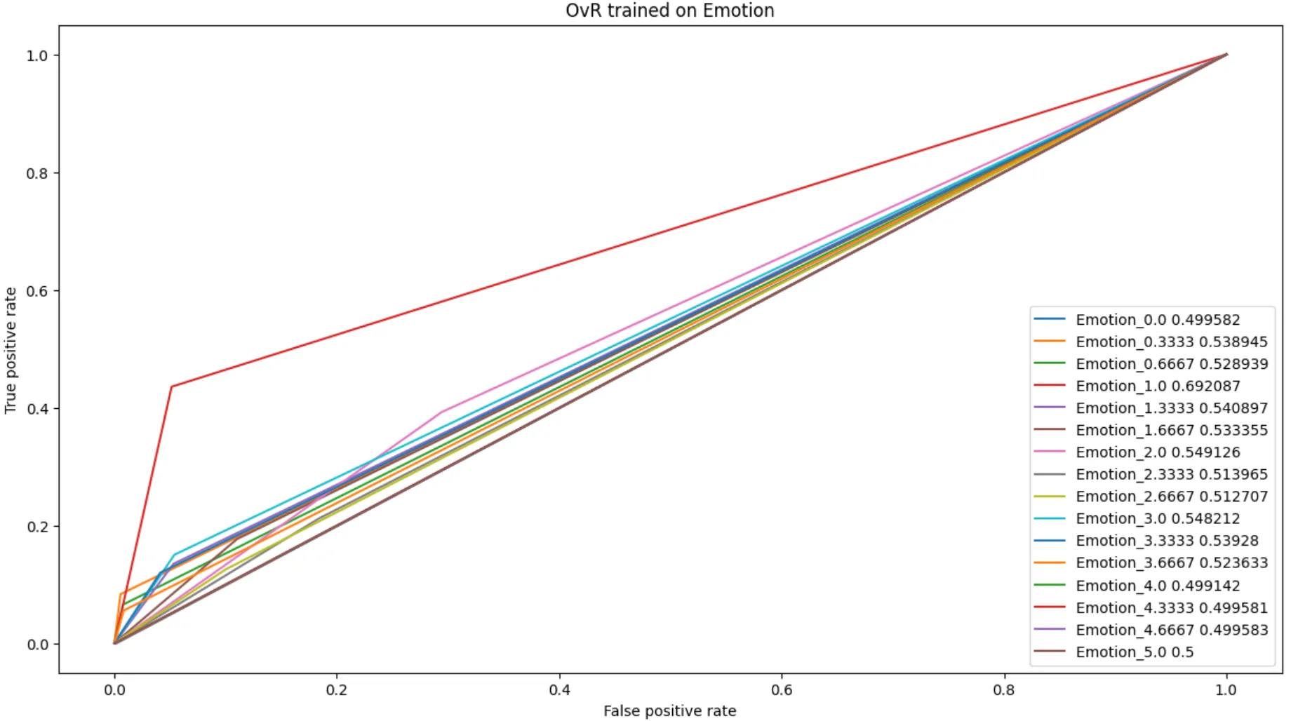
Unlike the figure of the Emotional Polarity baseline, most of the categories for this baseline for Emotional Intensity are higher than 0.5. This image looks like a better baseline model since this model works in classifying among most labels.
Baseline model for Empathy:
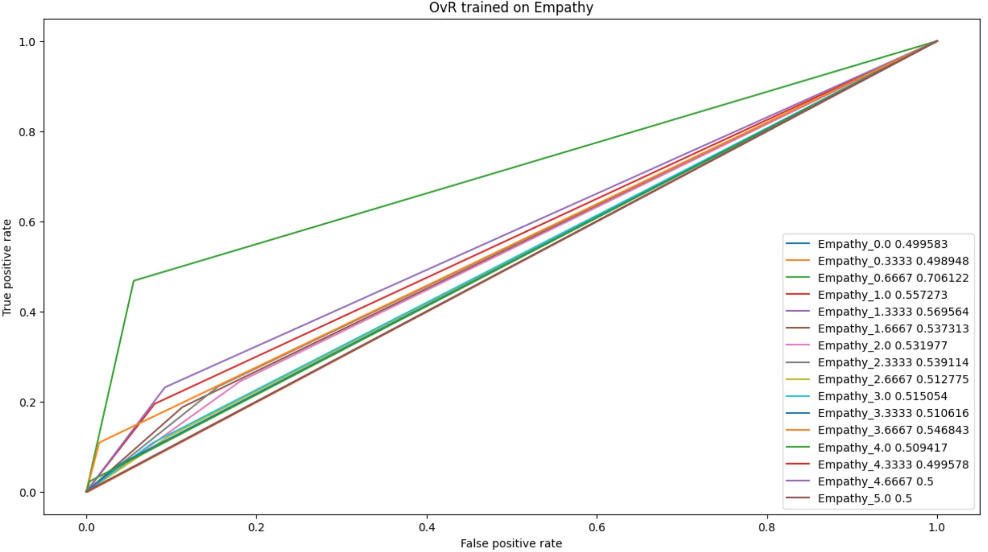
As can be seen in this figure, OvR doesn't perform that well but it is a nice fit to be a baseline model as well, and we can find Figure 3 and Figure 4 are similar which means the two models have similar discriminative power in distinguishing between positive and negative samples.
Baseline Performance Metrics:
| Emotional Polarity | Emotional Intensity | Empathy | |
|---|---|---|---|
| F1 Score | 0.386 | 0.205 | 0.185 |
| Accuracy | 0.386 | 0.205 | 0.185 |
| Pearson R score | 0.5074 | 0.512 | 0.516 |
Problem Formulation:
From our exploratory data analysis, we found that the Empathy, Emotional Polarity and Emotion scores are decimal values in the range [0, 5] for Empathy and Emotion and [0, 2] for Emotional Polarity. Based on the fact that the scores are float values, the problem can be formulated as a Regression problem.
Upon further exploring the data, it can be seen that rather than a continuous distribution, the Empathy, Emotional Polarity and Emotion scores take discrete values in their specific range. The possible scores for Empathy, Emotional Polarity and Emotion are as follows:
| Possible Values | |
|---|---|
| Empathy | 0.0, 0.3333, 0.6667, 1.0, 1.3333, 1.6667, 2.0, 2.3333, 2.6667, 3.0, 3.3333, 3.6667, 4.0, 4.3333, 4.6667, 5.0 |
| Emotion | 0.0, 0.3333, 0.6667, 1.0, 1.3333, 1.6667, 2.0, 2.3333, 2.6667, 3.0, 3.3333, 3.6667, 4.0, 4.3333, 4.6667, 5.0 |
| Emotional Polarity | 0.0, 0.3333, 0.5, 0.6667, 1.0, 1.3333, 1.5, 1.6667, 2.0 |
While formulating the problem as a Classification problem, it can also be noted that the individual classes have an ordering in them. For example, in the possible values in the Emotional Polarity scores shown in the table above, it can be seen that there is an ordering among the classes, i.e. 0.0 < 0.3333 < 0.5 < 0.6667 < ……… < 1.6667 < 2.0. This makes it possible to formulate this problem as an Ordinal Regression (also called Ordinal Classification Problem).
We tried all three methods (Regression, Classification and Ordinal Regression) to model our problem. Some details of each of them are as follows:
Regression:
During our initial attempts at modeling this problem, we focused on a regression based approach. We chose the Mean Squared Loss as our loss function and trained the model to minimize it for each of Empathy, EmotionalPolarity and Emotion. Since with a regression based approach the model outputs a value in a continuous distribution, during inference, we chose the class that is closest to the output of the model for our final prediction.
Classification:
While we experimented with regression for our initial models, we got better results with classification and ended up formulating most of our models as classification. The choice of loss function was Categorical Cross Entropy.
Ordinal Regression:
Since our categories have a strict ordering, we also attempted Ordinal Regression/Classification following the approach in the paper “A neural network approach to ordinal regression” by Cheng, J. (2007).
We first encoded the labels as a vector where all the labels before the actual label are also hot (basically similar to one-hot encoding but with all the zeros preceding the hot bit also set to 1). For example, we have the following possible labels for Emotional Polarity: [0.0, 0.3333, 0.5, 0.6667, 1.0, 1.3333, 1.5, 1.6667, 2.0].
Let’s say a sample has an emotional polarity score of 0.5. We encode the emotional polarity of this sample as [1, 1, 1, 0, 0, 0, 0, 0, 0]. We note that in this vector, the bits for the emotional polarity scores of 0.0 and 0.3333 are also on. This is basically implying that anything that has an emotional polarity of 0.5 will definitely have an emotional polarity of 0 and 0.3333.
After encoding the labels in this special vector, we used the MSE loss as our loss function to train our model (Cheng, J. stated in his findings that both Cross Entropy (classification) and Mean Squared Error (regression) losses work equally well).
During inference, we use the index of the rightmost class that has a sigmoid activation of over 0.5 as our prediction. For example, for the model’s output (sigmoid activated) of [0.9, 0.9, 0.6, 0.57, 0.4, 0.2], we choose the class of the 4th element i.e. 0.57 as our prediction (because 0.57 is the rightmost element that has a value of 0.5 or more).
We didn’t get better results than regular classification with this approach, so we did not use ordinal regression in our final models.
Things we tried:
We attempted a number of different models and architectures to solve our classification problem. Rather than choosing a single model and performing hyperparameter tuning on it, we chose to focus more on experimenting with different models and comparing their performances.
To make sure that we were comparing apples to apples and not oranges, and to make sure that any improvement in the performance came from mostly from the model architecture and not from the hyperparameter tuning aspect of training, we fixed our hyperparameters for our Transformer models to the following settings to compare different approaches:
| Parameter | Value | Note |
|---|---|---|
| Number of Epochs | 3 | After about 3 epochs, we found that most of our models started to overfit |
| Learning Rate | 1e-5 | |
| Batch Size | 8 | |
| Weight Decay | 0.01 | |
| Warmup steps | 500 | |
| Max Token Length | 96 | 96 was good enough for our speech-turn data |
Fine tuning a Base RoBERTA model with a classification head
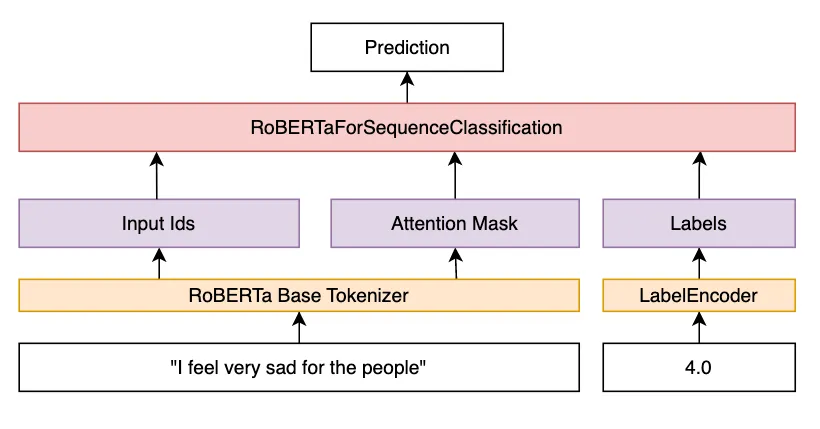
RoBERTa is a transformer-based language model, and is an extension of the popular BERT model. Before doing anything fancy, we wanted to see how a minimally tuned basic RoBERTa model would perform in our classification task. We used the Sequence Classification class of “roberta-base” from huggingface and changed the number of categories of the classification head to match ours and fine-tuned it for a few epochs.
Feature-based approach with RoBERTA
It was mentioned in the BERT paper that the authors found better results in classification by concatenating the hidden states of the last 4 layers of BERT instead of using just the last hidden state. We thought this could be a viable approach and attempted it with RoBERTa.
With this feature-based approach, we tried two different methods:
-
Using the hidden states while freezing the RoBERTa model
Just as in the previous approach, we configured RoBERTa to output all the hidden states and not just the last hidden state. But this time, we did not freeze the pertained model. The model was trained in a similar fashion as the previous approach.
- Using the hidden states while fine-tuning the pretrained model
Just as in the previous approach, we configured RoBERTa to output all the hidden states and not just the last hidden state. But this time, we did not freeze the pertained model. The model was trained in a similar fashion as the previous approach.
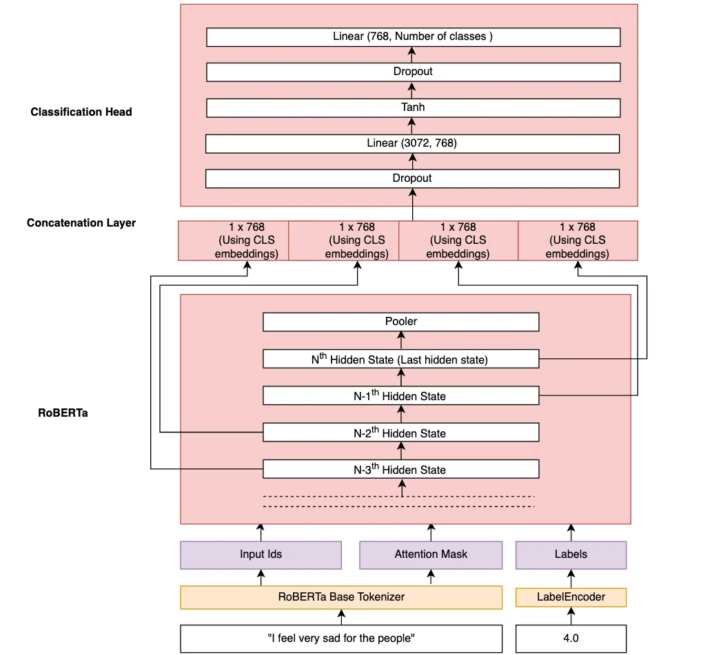
We found that not freezing the weights of RoBERTa performed better than freezing the base RoBERTa model. However, overall, we did not see a notable improvement in our model’s overall performance compared to just fine-tuning a base RoBERTa and using the CLS token embeddings of the last hidden state.
Using a model pre-trained for Sentiment Analysis
As things like Empathy, Emotion and Sentiment are similar (not the same), we had a hypothesis that a model that is trained specifically for Sentiment analysis might perform better than a basic RoBERTa model. To test this hypothesis, we searched for various pre-trained Sentiment Analysis models on huggingface. We chose the mode “Twitter-roBERTa-base for Sentiment Analysis” from CardiffNLP because it was trained on a very large corpus of Twitter tweets for Sentiment Analysis. We tried fine-tuning this model for Empathy, Emotion and Emotional Polarity. While it did not perform as well as we expected on Empathy and Emotion, fine-tuning it for classifying Emotional Polarity gave us the best results out of all of our models for predicting Emotional Polarity.
Masked Language Modeling approach
While playing around with transformer models, we came across Masked Language Models in huggingface. Masked Language Model is a language model that predicts the missing words (the masked value) in a given sentence based on the context. By treating our labels as a part of the text, we tried framing our problem as a Masked Language Modeling problem. Here is a summary of how we did our modeling:
- Encoded each class as an alphabet. This was to make sure that each class was represented by a single character (we think this could be anything that is in the tokenizer’s vocabulary as long as it’s a single token). For example, for Emotional Polarity, we used the following encodings.
0 → "A", 0.333 → "B", …………….., 1.6667 → "H", 2.0 → "I"
- Created a masked speech-turn text.
For example, let’s say the sentence “That is such a sad news story” has an Emotional Polarity of 1.6667. We prepend the string “[[[[]]]] “ in front of it to get the masked speech-turn text, which now becomes “[[[[]]]] That is such a sad news story”.
Notice the signs “[[[[“ and “]]]]” that appear before and after the token. We added these irregular signs because we thought that enclosing the mask with the same pattern in all samples would help make better predictions because for all samples in the training data there is always a single alphabet (class) between A and I enclosed by these signs and because of this, probability-wise, the model will only predict characters from A to I (our encoded classes) for the mask.
- Tokenized the masked speech-turn text from 2. using a RoBERTa tokenizer (with special tokens enabled). For our labels for the mask, we used the encodings from step 1.
- Trained the Masked Language Model.
- Decoded the characters predicted by the masked language model (“A” to “I” for Emotional Polarity) back to the original classes and used them as our prediction.
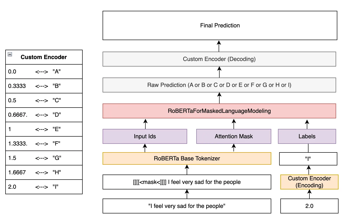
This model did not outperform the basic RoBERTa Sequence Classification approach. However, since the performances were similar, we decided to use this approach as our final model for Empathy and Emotion as we thought it was a more non-traditional approach.
RoBERTa with LSTM
We used word embeddings from RoBERTa as our input to a LSTM classifier (the weights of the pretrained RoBERTa were frozen) as one of our modeling approaches. We experimented with different architectures and parameters of the LSTM model (stacked/not stacked, unidirectional/bi-directional, etc) to try to improve our performance, but unfortunately this approach could not outperform the basic fine-tuned RoBERTa model.
Other experiments
Aside from the different kinds of models we tried, we also attempted a few other approaches to try to improve our models’ performance.
Data Preprocessing
The class distribution for each of Empathy, Emotion and Emotional Polarity was very imbalanced.
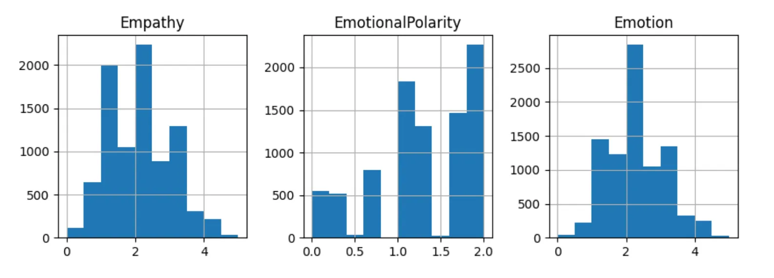
We attempted to remove the class imbalances by random undersampling and random oversampling using the imbalanced-learn library. However, we did not have a lot of success with either of these methods.
Data Augmentation
To introduce more variation to our speech-turn data and to increase the size of our training data, we performed data augmentation by paraphrasing the speech-turn level text. To do this, we used the Parrot paraphraser library. With this, we could increase the size of our training data to about 24,000, a 3X increase in our training data size. For each paraphrase, we copied the Empathy scores of the original text. We only trained for Empathy using this data because we thought that for labels other than Empathy (Emotion and Emotional Polarity), the choice of words in the paraphrase might impact the emotion intensity and polarity and therefore, for those two labels, copying the corresponding label from the original text would not be justified.
We could get a slight improvement in Empathy prediction performance with this approach.
Confident Learning
While exploring our training data, we found that we had some noisy labels (eg. having different scores for the same/similar text). We did some literature review on approaches that can be taken to reduce such noise in text data and came across the paper “Confident Learning: Estimating Uncertainty in Dataset Labels” by Northcutt et al. The paper introduces a framework that uses a probabilistic model to estimate the confidence or uncertainty of each label in a dataset. Northcutt et al. have also open-sourced a python library called cleanlab that can be used to easily detect noisy labels in datasets.
We used this library to find noisy labels in our training data and found that this library indeed helps detect data points that are outliers and that are easy to be misclassified by the models to a certain extent. It gives a number estimate of the “label quality” with a lower number implying bad quality and a high number implying the label is good. After detecting weak labels from the dataset, we dropped samples whose label quality was below a certain threshold and trained our models with the higher quality data points. The performance does seem to increase a little bit, but not by a large margin that we were expecting.
Label Smoothing
Since we framed most of our models as classification, we attempted to boost performance by applying label smoothing on our data. Label smoothing is a regularization technique that helps a model to generalize better in classification tasks. Usually for classification tasks, since we use one-hot encodings as true labels and sigmoid activations as predictions, the model can never acquire a zero loss because the sigmoid function can never output exactly 0 or 1. Apparently this hard boundary between the classes makes the model make overconfident predictions. Label smoothing is a way of addressing this issue by smoothing the true labels and changing the one-hot vector to a more smooth representation eg. [0, 0, 1] → [0.05, 0.05, 0.9] This reduces the overconfidence problem and gives a chance for the model to predict the other classes as well.
Since we adopted label smoothing late in our project, we have not been able to thoroughly evaluate the impact of applying label smoothing in our performance.
Cosine annealing with hard restarts
We found that sometimes resetting the learning rate and epochs and training the same model instance further helped our model converge better. We think this was because of the high learning rate at the starting epochs (because of the resetting) that helped the model go over a local minima that it had gotten stuck at the end of the previous epoch (where the learning rate has decayed to a small value). While researching for approaches to handle this, we found the concept of cosine annealing with restarts. The idea is to use the cosine wave as a decay function and once a certain rate is reached, the learning rate is restarted (reset) to the original value, from where it starts to decay again. We used the Huggingface’s Trainer class’s “lr_scheduler_type” option to use cosine annealing with hard restarts in our models.
Our Final Models:
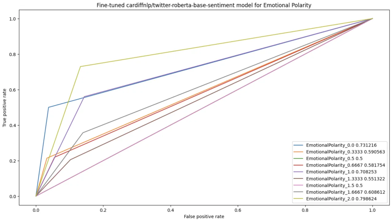
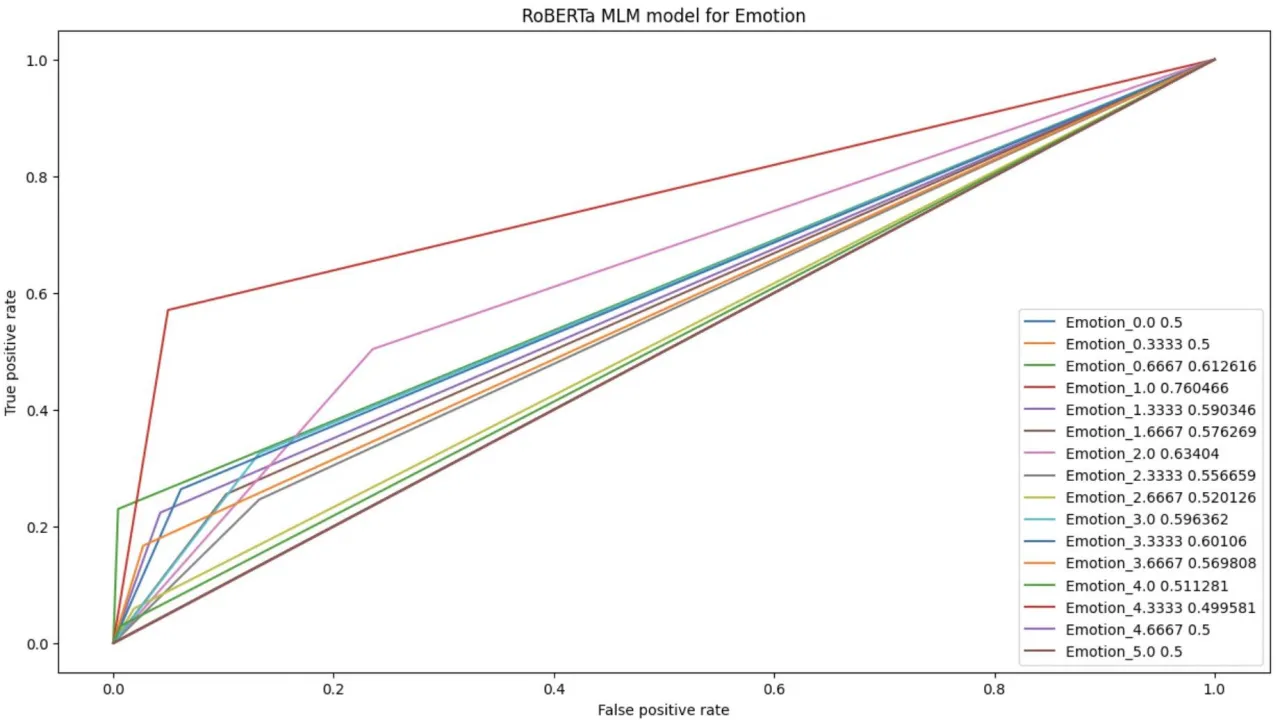
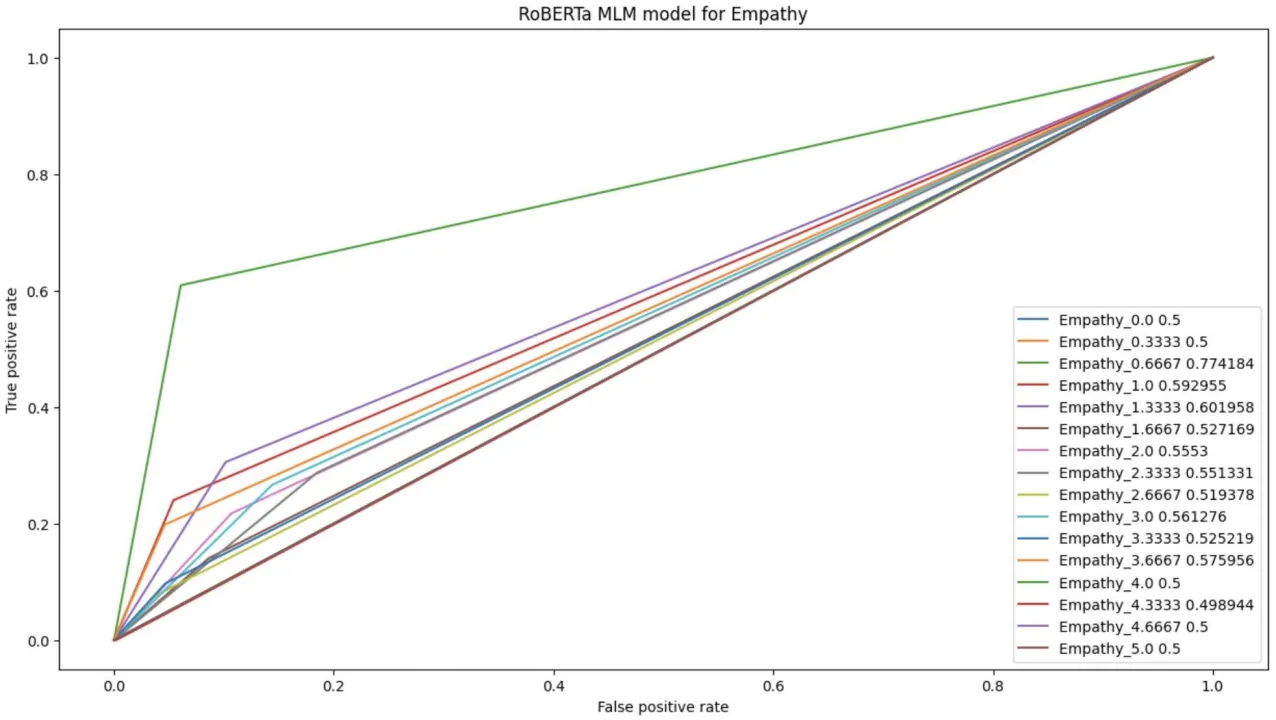
As a result of all the modeling and optimization approaches mentioned above for predicting EmotionalPolarity, Emotion and Empathy, we selected one model each for Empathy, Emotional Polarity and Emotion as our final models. For predicting Emotional Polarity, fine-tuning the pre-trained CardiffNLP Sentiment Analysis outperformed all of our other models by a large margin, so we picked that as our Emotional Polarity classifier. For Empathy and Emotion, we chose the models that we trained using the Masked Language Modeling approach because we thought this was an interesting approach and also because its performance was comparable to fine-tuning a RoBERTa model for classification.
The ROC curves and the final metrics of each of our best models are as follows:
Emotional Polarity:
| Pearson R Score | F1 Score | Accuracy | |
|---|---|---|---|
| Final model | 0.7689 | 0.4667 | 0.4667 |
| Baseline model | 0.5074 | 0.3860 | 0.3860 |
Emotional Intensity:
| Pearson R Score | F1 Score | Accuracy | |
|---|---|---|---|
| Final model | 0.7452 | 0.2888 | 0.2888 |
| Baseline model | 0.5115 | 0.2050 | 0.2050 |
Empathy:
| Pearson R Score | F1 Score | Accuracy | |
|---|---|---|---|
| Final model | 0.6631 | 0.2200 | 0.2200 |
| Baseline model | 0.5160 | 0.1850 | 0.1850 |
Overall, with our final models, the F1 score, Accuracy and Pearson R scores increased with respect to the baseline model. Based on the classwise ROC curves listed below, we can see that the final models have varying degrees of success based on the class. For example, our model for predicting Emotional Polarity has AUC of 73, 70 and 79 for Emotional Polarity of 0.0, 1.0 and 2.0 respectively. However, it has comparatively lower AUC (mostly between 0.5 to 0.6) for other classes, implying that the model can easily classify some classes while it has a harder time classifying some other classes.
Conclusion:
This study aimed to predict perceived Empathy, Emotional Polarity, and Emotional Intensity in conversation using three main approaches: fine-tuning a Base RoBERTa model, a feature-based approach using RoBERTa, and a Masked Language Modeling approach with RoBERTa. Instead of focusing on hyperparameter tuning, we focused on comparing the different models against each other and finding which model is inherently better, with hyperparameters being the same. Our findings suggest that fine-tuning a transformer pre-trained on sentiment analysis achieved the best results for classifying Emotional Polarity. For predicting Emotion and Empathy, fine-tuning a RoBERTa model alone yielded decent outcomes. Additionally, we devised a method to use Masked Language Modeling for classification by manipulating the input data and leveraging the Masked Language Model to predict label values. Although the results were not exceptional, the performance was comparable to fine-tuning a base RoBERTa Sequence Classification model. Hence, we selected the Masked Language Model for predicting Empathy and Emotion scores in the WASSA shared task due to its intriguing nature.
Overall, there was a significant improvement in accuracy and F1 scores across all three categories, with Emotional Polarity accuracy more than doubling. Furthermore, the Pearson R score enhanced for all categories, with Emotional Polarity exhibiting the largest increase. These results emphasize the potential of natural language processing and machine learning techniques to accurately predict and comprehend the complex emotions conveyed in human conversations. The impact of computers understanding emotions and empathy is intricate and multifaceted.
Limitations:
For as much as we were able to accomplish in formulating solutions for our task, there were still limitations we encountered which prevented us from creating as high-performing models as we had hoped. For one, it appears the data is imbalanced, with some scores having a very high representation in the dataset while some scores had only a handful of samples. This could also have been the reason that the class-wise ROC curves were very different for different classes. We also suspect that there was some noise in the labels, as well. For example, speech-turn text like “Bye bye” has higher scores in emotional polarity, emotional intensity, and empathy than another turn with the text “Bye”, despite the two turns’ text differing very little. Annotations like this could lead the model to believe such similar text to differ more than the average person might think, which could have resulted in training toward inaccurate predictions. Finally, less technically, we were computationally limited in our use of Google Colab’s free-trial GPU. While this did provide a better system of collaboration between us, we would occasionally get kicked off the GPU system time we were allocated, resulting in us either having to wait until our allotted time refreshed, or needing to create new Google accounts. If we were not limited in these ways, our model might have performed better with better data to train on, and we might have used our time more efficiently without needing to deal with Google Colab’s GPU limitations.
References:
Barbieri, F., Camacho-Collados, J., Espinosa Anke, L., & Neves, L. (2020). TweetEval: Unified Benchmark and Comparative Evaluation for Tweet Classification. In Findings of the Association for Computational Linguistics: EMNLP 2020 (pp. 1644-1650). Association for Computational Linguistics.
Cheng, J. (2007). A neural network approach to ordinal regression (Version arXiv:0704.1028v1). Retrieved from https://doi.org/10.48550/arXiv.0704.1028
Damodaran, P. (2021). Parrot: Paraphrase generation for NLU (Version v1.0) [Computer software]. Retrieved from https://github.com/PrithivirajDamodaran/Parrot
Devlin, J., Chang, M. W., Lee, K., & Toutanova, K. (2018). BERT: Pre-training of Deep Bidirectional Transformers for Language Understanding. arXiv preprint arXiv:1810.04805.
Liu, Y., Ott, M., Goyal, N., Du, J., Joshi, M., Chen, D., ... & Stoyanov, V. (2019). RoBERTa: A robustly optimized BERT pretraining approach. arXiv preprint arXiv:1907.11692.
Northcutt, C. G., Jiang, L., & Chuang, I. L. (2019). Confident Learning: Estimating Uncertainty in Dataset Labels (Version 6). arXiv preprint arXiv:1911.00068